Protocols are constantly in search of ways to achieve more “bang for the buck.”
Sometimes abbreviated as !4$ - this phrase originated in the 1950s and quite literally referred to military firepower and weaponry. In DeFi, a bigger protocol bang for voter incentive buck can be achieved via honing in on an incentive’s price range.
Part-1 of this vote incentives mini-series introduced the economic principles (or flywheel) at play within the governance wars and identified several variables responsible for the correlation between incentive volume and value.
Part-2 discussed the differences between fixed & variable voting incentives and also identified clusters and habits of voters while starting to quantify the maximum final price range of a specific incentive.
To further define the expected price range for future and ongoing voting incentives, this part of the mini-series will demonstrate the efficiency of probabilistic models based on historical data.
Since we conduct our research in a theoretical and fundamental framework, it should be possible to apply our findings to any gauge ecosystem. This part of the research will be based on the data extracted from Balancer/Aura.
Hidden Markov Model (MDP)
In mathematics, a Markov decision process (MDP) is a discrete-time stochastic control process. It provides a mathematical framework for modeling decision making in situations where outcomes are partly random and partly under the control of a decision maker. MDPs are useful for studying optimization problems in economics.
A Markov process is a sequence of certain states where the probability of a certain state happening next is only dependent on the current state we are in.
Studying voting incentives, all states correspond to a specific $/vote ratio. Thus, we have a wide range of states and we don't know what those states are exactly, but we have some observable variables. This is where the Hidden Markov Model comes in.
Maximum likelihood estimation (MLE)
The first step of our research will be to define the probabilities that are the most likely to be correct for each state of our $/vote range. A popular way to do this is called Maximum Likelihood Estimation (MLE)
Maximum likelihood estimation (MLE) is a statistical method of estimating the parameters of an assumed probability distribution, given some observed data. This is achieved by maximizing a likelihood function so that, under the assumed statistical model, the observed data is most probable.
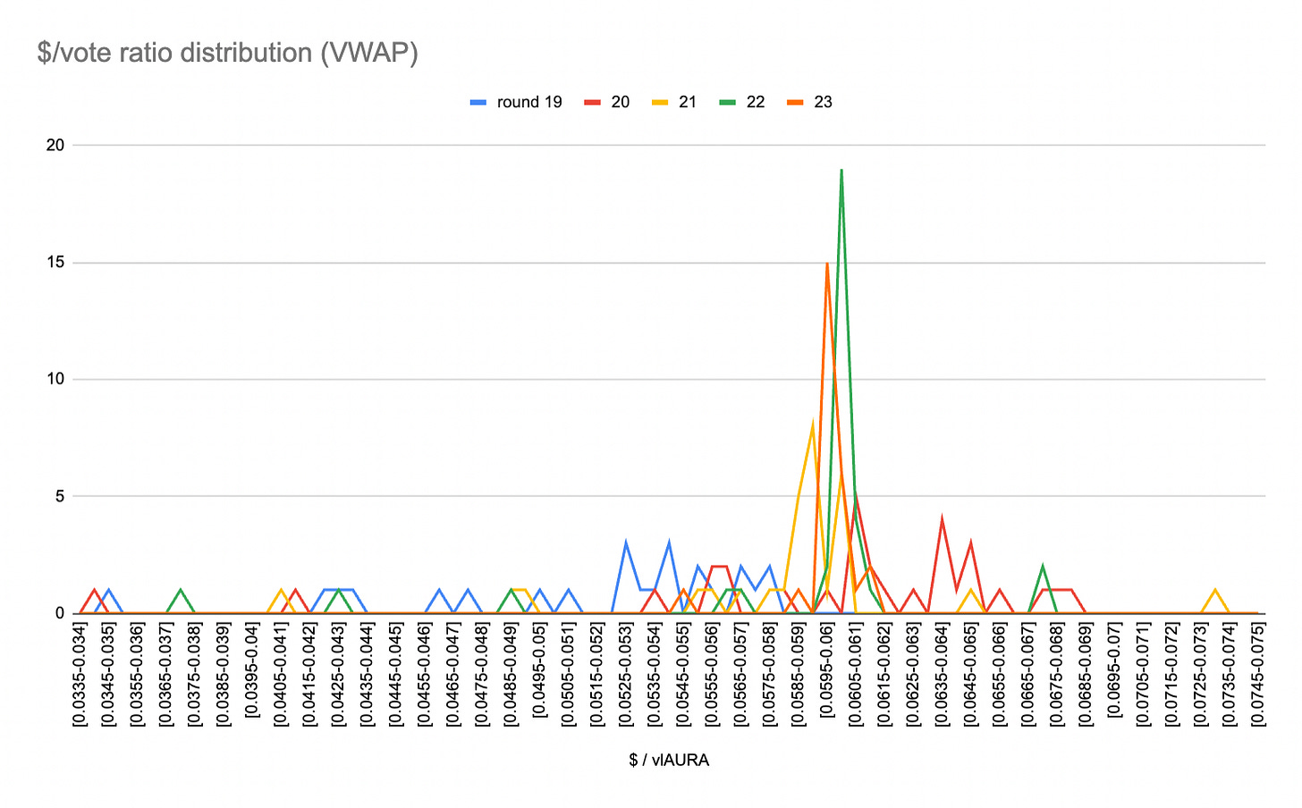
When analyzing the distribution of $/vote ratios of voting incentives, it is possible to smoothen the volatility between each round based on:
The correlation between volume and value that we highlighted in part 1
The intrinsic value of the discounted directed emissions.
Using this method, it is possible to display the visualization below, showing that the $/vote distribution is following a normal law.
Thanks to this demonstration, we can consider a model law of standard deviation σ with expectancy μ. For each case, we determine the heights H(i) corresponding to the value of the density function in xi. The likelihood L is then defined as the product of the heights.
L = (H1 * H2 * H3 * … * Hn)
Because we compare various set of data representing each rounds, we are given a distribution 𝑓(𝑥𝑖,𝑦𝑖;𝛼,𝛽) and joint probability function 𝐹(𝑥1,...,𝑥𝑁,𝑦1,...,𝑦𝑁;𝛼,𝛽)
The first order derivatives are :
∂𝐹∂𝛼 and ∂𝐹∂𝛽
And the first order conditions :
∂𝐹 / ∂𝛼 =0 and ∂𝐹 / ∂𝛽 =0
Maximum likelihood estimation is a multivariable function. For a point to be considered the local minimum or maximum point of a function it must be a stationary point, i.e. the point at which all first order partial derivatives are zero.
The intuition transfers from one variable function. The stationary point is the point where the derivative is zero. For multivariable functions the derivative is a vector which is equal to zero, when all elements are zero.
Given that the highest likelihood is the optimal data sample to choose dispersion parameters expectancy & standard deviation, we will be using data from Round 20 to compute the next steps.
Let X be a real random variable, with the distribution D {\mathcal {D}}_{\theta }, of parameter \theta unknown. For the sake of simplicity and to stick with the Markov decision process, we will define a function f with a discrete law.
Because we want X to be a discrete variable to be able to write f(x ; θ) = Pθ(X = x) , which is the probability that X = x, we will use the average value of each range of Xi.
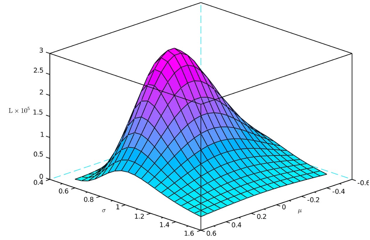
For our example, if we plot the likelihood value L as a function of the parameters μ and σ, we obtain a surface whose maximum is in (μ = ? , σ = ?). Finding this maximum is a classical optimization problem.
“General representation of likelihood maxima”
The estimator obtained by the maximum likelihood method is:
Convergent
Asymptotically efficient because it reaches the Cramér-Rao bound
Asymptotically distributed according to a normal distribution
In conclusion, we have demonstrated that the voting incentives market matches the conditions to be analyzed through the scope of probabilistic models in order to quantify and forecast future $/vote ranges.
The methods and strategies outlined in our ‘Vote Incentive Pricing’ mini-series can be utilized across any gauge ecosystem by protocols and individual participants to achieve the biggest bang for your buck.


